
by TJ Murphy, @teej_m on Twitter This article was originally published on Towards Data Science on Jan 18, 2019.
It always starts with an innocent observation. “We get a lot of traffic from Boston,” your boss remarks. You naturally throw out a guess or two and discuss why that might be. Until your boss drops the bomb —
“Can you dig into that?”
Darn it. You walked right into that one.
Now you’re in a predicament. You know Google Analytics has traffic by geographic location, but that’s not gonna cut it. If you want to report on those retention rates, lifetime values, or repeat behaviors by geo, you need something you can query with SQL, something that lives in your data warehouse. But you don’t have anything like that. You know there’s user IP addresses in your log data, you just need to turn them into locations. But Redshift doesn’t have a way to do that.
What you need is geolocation using IPs, aka GeoIP. The place folks commonly start is MaxMind, mostly because it’s the first Google result for “GeoIP”. Together we will use their IP-to-City dataset to enrich our log data and determine what city and country our users are from. We will use MaxMind data because it’s reliable and robust. Also it’s free. One less thing to bother your boss about.
So off we go to download
MaxMind’s GeoLite City data.
Upon opening the zip, we find a number of CSV files, the most important among
them being GeoLite2-City-Blocks-IPv4.csv. If we peek inside, this is what we
see:
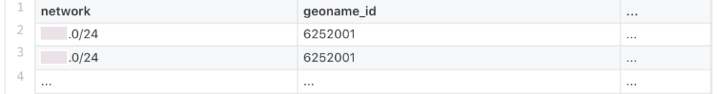
Right away we notice a problem — this data has something that looks like an IP but has a slash and an extra number at the end. This is an IP network represented in CIDR notation and it represents a range of IPs. It’s composed of an IP, a slash, and a number after the slash called a subnet mask. It’s like how you might describe a street of physical addresses in New York City by saying “The 500 block of west 23rd street.”
If we had the network X.Y.Z.0/24 that would mean “every IP that starts with
X.Y.Z. and has any number between 0 and 255 at the end. In other words, any IP
between X.Y.Z.0 and X.Y.Z.255. So if we observed a user with the IP
X.Y.Z.95, that would fall in the network X.Y.Z.0/24 and thus is located in
geoname_id of 6252001. A subnet mask can be any number between 1 and 32 and
the smaller the number, the wider the network.
If this MaxMind table were in Redshift, how would we join to it? Redshift doesn’t include any handy network address types likes modern Postgres or INET functions like MySQL. Instead we will use knowledge of the math behind IPs to do the work ourselves.
You can think of an IP as a fancy representation of a really big number. The IP
1.2.3.4 is really just 16,909,060 under the hood. Similarly, IP networks are
just ranges of really big numbers. The network 1.2.3.0/24 is a range that
starts with 16,909,056 and ends with 16,909,311. We will use this to our
advantage. To do so, we need a way to convert IPs and IP networks to numbers.
Using the geoip2-csv-converter tool provided by MaxMind, we will add the integer range representation of each network to our CSV.
# Download the converter tool from Github
curl -o geoip2-csv-converter-v1.1.0-darwin-amd64.tar.gz \
     -L https://github.com/maxmind/geoip2-csv-converter/releases/download/v1.1.0/geoip2-csv-converter-v1.1.0-darwin-amd64.tar.gz
tar xvf geoip2-csv-converter-v1.1.0-darwin-amd64.tar.gz

# Use the tool to add integer range columns to our CSV
./geoip2-csv-converter-v1.1.0/geoip2-csv-converter \
 -block-file=GeoLite2-City-CSV_20190108/GeoLite2-City-Blocks-IPv4.csv \
 -output-file=GeoLite2-City-Blocks-IPv4-with-ranges.csv \
 -include-cidr \
 -include-integer-range
gzip GeoLite2-City-Blocks-IPv4-with-ranges.csv
Note that I’m using the 20190108 version. MaxMind updates this data set
weekly, so your version may be different.
After uploading our modified CSV to S3, we can COPY it into Redshift.
-- Create Maxmind IP to geo table in Redshift
-- https://dev.maxmind.com/geoip/geoip2/geoip2-city-country-csv-databases/
CREATE TABLE maxmind_ipv4_to_geo (
  network VARCHAR
, network_start_integer BIGINT
, network_last_integer BIGINT
, geoname_id INTEGER
, registered_country_geoname_id INTEGER
, represented_country_geoname_id INTEGER
, is_anonymous_proxy BOOLEAN
, is_satellite_provider BOOLEAN
, postal_code VARCHAR
, latitude NUMERIC
, longitude NUMERIC
, accuracy_radius INTEGER
);
-- Copy our CSV into the Maxmind table
COPY maxmind_ipv4_to_geo
FROM 's3://path/to/your/data/GeoLite2-City-Blocks-IPv4-with-ranges.csv.gz'
CREDENTIALS '...YOUR_CREDENTIALS_GO_HERE...'
CSV
GZIP
IGNOREHEADER AS 1
;
Now let’s write a function to convert IPs to really big numbers. Here’s a simple
one written in SQL. We will call it inet_aton after the Linux utility that
does the same thing. “inet” stands for “internet” and “aton” means “Address TO Number”. Linux folks like to keep things short and sweet.
-- Create a function to convert IPs to numbers. Named after the linux inet_aton utility.
CREATE FUNCTION f_inet_aton(VARCHAR)
RETURNS BIGINT IMMUTABLE as $$

  SELECT (
            SPLIT_PART($1, '.', 1)::BIGINT * POW(256, 3) +
            SPLIT_PART($1, '.', 2)::BIGINT * POW(256, 2) +
            SPLIT_PART($1, '.', 3)::BIGINT * POW(256, 1) +
            SPLIT_PART($1, '.', 4)::BIGINT * POW(256, 0)
         )::BIGINT

$$ LANGUAGE sql;
The last thing we need is to load the MaxMind CSV that contains a lookup from
geoname_id to an actual place on earth. We will gzip it for speed, upload the
GeoLite2-City-Locations-en.csv.gz file to S3, and COPY it to a table.
Some quick pointers on Redshift optimization. For a small, commonly joined
dimension table like this, I recommend DISTSTYLE ALL. This makes a copy of the
table on every node in your cluster, eliminating a data transfer step during
joins. I also define our join column as a SORTKEY to speed things up.
-- Create Maxmind geo to city table in Redshift
CREATE TABLE maxmind_geo_to_city (
  geoname_id INTEGER
, locale_code VARCHAR
, continent_code VARCHAR
, continent_name VARCHAR
, country_iso_code VARCHAR
, country_name VARCHAR
, subdivision_1_iso_code VARCHAR
, subdivision_1_name VARCHAR
, subdivision_2_iso_code VARCHAR
, subdivision_2_name VARCHAR
, city_name VARCHAR
, metro_code VARCHAR
, time_zone VARCHAR
, is_in_european_union BOOLEAN
)
DISTSTYLE ALL
SORTKEY (geoname_id)
;
-- Copy our CSV into the Maxmind table
COPY maxmind_geo_to_city
FROM 's3://path/to/my/data/GeoLite2-City-Locations-en.csv.gz'
CREDENTIALS '...YOUR_CREDENTIALS_GO_HERE...'
CSV
GZIP
IGNOREHEADER AS 1
;
Now we have everything we need to enrich our logs with location data using GeoIP. Almost everything.
Redshift Is Hard
If we join our new MaxMind GeoIP tables to our log data, we will immediately run into a problem. Suppose I have some bare bones access logs and try to calculate the top 50 regions by traffic.
CREATE TABLE access_logs (
  ip_address VARCHAR,
  created_at_utc TIMESTAMP,
  user_id INTEGER
);
If you ran this query, you’re going to have a bad time. You query will be running for minutes and you’ll start to sweat. Meanwhile your Redshift admin will be hunting for the individual who took down her cluster. Don’t be that person.
 SELECT mm_city.city_name
      , mm_city.country_name
      , COUNT(*) AS traffic
   FROM access_logs AS log
   LEFT JOIN maxmind_ipv4_to_geo AS mm_geo
     ON f_inet_aton(log.ip_address) BETWEEN mm_geo.network_start_integer
                                        AND mm_geo.network_last_integer
   LEFT JOIN maxmind_geo_to_city AS mm_city
     ON mm_geo.geoname_id = mm_city.geoname_id
  GROUP BY 1, 2
  ORDER BY 3 DESC
  LIMIT 50
;
What’s wrong with this query? A quick peek at the EXPLAIN plan, the list of
steps Redshift takes to execute the query, tells all.
Suppose you ran an ice cream shop with millions of delicious flavors. What if
each customer in line had to taste-test every single flavor before they could
choose one? That’s what happens if we attempt to combine our log data
(customers) to the MaxMind data (flavors) directly using our BETWEEN join
(taste-test). This results in a
nested loop join,
one of the quickest ways to make a database cry.
To speed up our ice cream shop, we are going to organize it into distinct sections — the chocolates over here, the vanillas over there, and a special spot for the minty flavors. Laid out this way, customers head to the one section that matches their preference. Once there they taste-test a minuscule number of flavors in comparison to before.
Creating an optimized GeoIP lookup table
We will build a new table in Redshift that will replace maxmind_ipv4_to_geo
that’s optimized for GeoIP lookups. We will organize it into distinct sections
using the first half of the IPs and place each network into it’s proper section.
Some networks are wide enough that they will go into more than one section.
These sections act almost like a database index, allowing Redshift to narrow
down which networks to check for each IP. Using a little bit-twiddling magic, we
take our table and convert it into one that’s fast and optimized.
-- Create a helper table to allow us to enumerate from 0-255.
-- This is a quick hack to generate a table with just the numbers 0 to 255 in it.
 CREATE TEMPORARY TABLE range_0_to_255 AS
 SELECT ROW_NUMBER() OVER () - 1 AS num
   FROM maxmind_geo_to_city
  ORDER BY 1
  LIMIT 256
;

-- Create the special lookup table
CREATE TABLE maxmind_ipv4_lookup
DISTSTYLE ALL
AS
 SELECT octet_1.num || '.' || octet_2.num AS first_16_bits
      , mm.network_start_integer
      , mm.network_last_integer
      , mm.network
      , mm.geoname_id
   FROM maxmind_ipv4_to_geo mm
   JOIN range_0_to_255 octet_1
     ON octet_1.num BETWEEN (mm.network_start_integer & f_inet_aton('255.0.0.0')) >> 24
                        AND (mm.network_last_integer & f_inet_aton('255.0.0.0')) >> 24
    JOIN range_0_to_255 octet_2
      ON octet_2.num BETWEEN (mm.network_start_integer & f_inet_aton('0.255.0.0')) >> 16
                         AND (mm.network_last_integer & f_inet_aton('0.255.0.0')) >> 16
;
With our lookup table created, we can take another crack at our analysis. In our
query, we swap out maxmind_ipv4_to_geo for maxmind_ipv4_lookup and add a new
join condition. We will extract the first half of each IP with the regex
REGEXP_SUBSTR(log.ip_address, '\\d+\.\\d+') and match it to it’s appropriate
section in the table mm_geo.first_16_bits. Then we check which network it
belongs in using the integer representation of the IP and network. With this
optimization, our query returns quickly with no nested loop join in sight!
 SELECT mm_city.city_name
      , mm_city.country_name
      , COUNT(*) AS traffic
   FROM access_logs AS log
   LEFT JOIN maxmind_ipv4_lookup AS mm_geo
     ON REGEXP_SUBSTR(log.ip_address, '\\d+\.\\d+') = mm_geo.first_16_bits
    AND f_inet_aton(log.ip_address) BETWEEN mm_geo.network_start_integer
                                        AND mm_geo.network_last_integer
   LEFT JOIN maxmind_geo_to_city AS mm_city
     ON mm_geo.geoname_id = mm_city.geoname_id
  GROUP BY 1, 2
  ORDER BY 3 DESC
  LIMIT 50
;
And with that, you’re ready to start your analysis. You can use this lookup
table to join to any other in Redshift with an IP. Just remember to always
include the join to first_16_bits as that’s the magic behind the approach.
This approach is inspired by a paper I read about optimizing IP lookups in a network appliance. I unfortunately can’t find the paper anymore. This post is a result of porting that solution to Redshift and iterating to reduce it to something simple and performant.
Thanks to the dbt Slack for inspiring this post, Julian Ganguli for working with some early code, and to Nick James for reading an early draft.
by TJ Murphy, @teej_m on Twitter This article was originally published on Towards Data Science on Jan 18, 2019.